course-notes
COMP3311 Notes
Written by Jeremy Le on April 27 2023. Heavily inspired by Luka Kerr’s Notes.
Table of Contents
- Data Modelling
- Entity-Relationship Data Modelling (ER Model)
- Relational Model
- Relational DMBSs
- Programming With SQL
- Programming With Databases
- Relational Design Theory
- Normalisation
- Relational Algebra
- DMBS Architecture
- Transactions
Data Modelling
Data modelling is a design process which converts requirements into a data model.
The aims of data modelling are to:
- describe what information is contained in the database
- describe relationships between data items
- describe constraints on data
Entity-Relationship Data Modelling (ER Model)
The world is viewed as a collection of inter-related entities.
ER has three major modelling constructs:
- Attribute: data item describing a property of interest
- Entity: collection of attributes describing object of interest
- Relationship: association between entities (objects)
ER Diagrams
ER diagrams are a graphical tool for data modelling.
An ER diagram consists of:
- a collection of entity set definitions
- a collection of relationship set definitions
- attributes associated with entity and relationship sets
- connections between entity and relationship sets
Key = set of attributes that uniquely identifies each entity instance
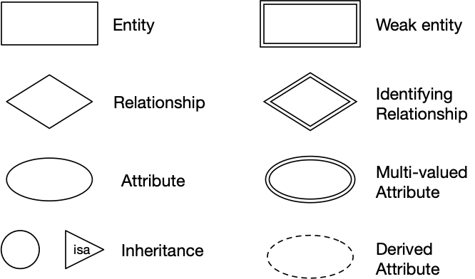
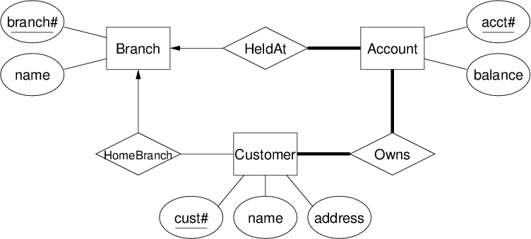
ER design elements:
Entities
An entity can be viewed as either a set of entities with the same set of attributes or an abstract description of a class of entities.
Relationship Sets
A relationship is an association among several entities. A relationship set is a collection of relationships of the same type.
Relationships contain
- Degree: the number of entities involved in the relationship
- Cardinality: the number of associated entities
- one-to-one (
[entity]<--(rel)-->[entity]) - one-to-many (
[entity]<--(rel)---[entity]) - many-to-many (
[entity]---(rel)---[entity])
- one-to-one (
- Participation: whether every entity must be in the relationship
- total participation (thick line)
- partial participation (thin line)
Class Hierarchies
ER also implements super-class / sub-class hierarchies
- both super- and sub-classes consist of entities
- super-class has common properties of all entities in hierarchy
- sub-classes can add extra properties to specialise
- entities in super-class may have corresponding entities in sub-class
- sub-classes can be
- disjoint (entities are members of only one sub-class)
- overlapping (entities are members of several sub-classes)
Relational Model
A relational model contains
- Tuples are collections of values
- Relations are set of tuples
- Constraints are logical statements on valid data
Tuples correspond to entities whilst relations correspond to entity sets and relationships.
Constraints
There are different types of constraints
- unique = value of attribute is unique in relation
- key = chosen unique attribute to distinguish tuples
- domain = type of attribute, restrictions within type
- referential integrity = foreign key
- tuple in relation R has attribute F
- whose value corresponds to key attribute K in relation S
Relational DMBSs
A relational database management system (RDBMS)
Managing Databases
# Create a new, empty database
$ createdb dbname

# Drop and remove all data from a database
$ dropdb dbname

# Dump the contents of a database
$ pg_dump dbname > dumpfile

# Restore the contents of a database dump
$ psql dbname -f dumpfile
SQL
SQL is a Data Definition Language that can formalise relational schemas.
CREATE TABLE TableName (
  attrName1 domain1 constraints1,
  attrName2 domain2 constraints2,
  ...
  PRIMARY KEY (attri, attrj,...)
  FOREIGN KEY (attrx, attry,...)
              REFERENCES
              OtherTable (attrm, attrn,...)
);
Syntax
-- Comments are after two dashes

-- Identifiers are alphanumeric and can be inside double quotes
-- Identifiers are case insensitive
"An Identifier", AnIdentifier

-- There are many keywords
CREATE, SELECT, TABLE, WHERE

-- Strings are inside single quotes
'a string'

-- Numbers are similar to C
1, -5, 3.14159

-- There are multiple types
integer, float, char(n), varchar(n), date

-- There are multiple operators
=, <>, <, <=, >, >=, AND, OR, NOT
Managing Tables
-- Create a table with attributes and constraints
CREATE TABLE table (Attributes + Constraints)

-- Modify a table
ALTER TABLE table TableSchemaChanges

-- Drop a table
DROP TABLE table(s) [ CASCADE ]

-- Truncate a table
TRUNCATE TABLE table(s) [ CASCADE ]
Managing Tuples
-- Insert into a table
INSERT INTO table (Attrs) Values Tuple(s)

-- Delete from a table
DELETE FROM table WHERE condition

-- Update a table
UPDATE table SET AttrValueChanges WHERE condition
where
Attrs=(attr1, attr2, ..., attrn)Tuple=(val1, val2, ..., valn)AttrValueChangesis a comma separated list ofattrname = expression
Types
-- Define own constrained type
CREATE DOMAIN Name AS Type CHECK (Constraint)

-- Define tuple type
CREATE TYPE Name AS (AttrName AttrType, ...)

-- Define enumerated type
CREATE TYPE Name AS ENUM ('Label', ...)
String Comparison
a < bcompares stringsaandbusing dictionary ordera LIKE patternmatches stringato pattern%matches anything_matches a single char
PostgreSQL provides regexp-based pattern matching.
-- ~ and !
Attr ~ 'RegExp'     -- Matches 'RegExp'
Attr !~ 'RegExp'    -- Doesn't match 'RegExp'

-- ~* and !~*
Attr ~* 'RegExp'    -- Matches 'RegExp' case-insensitive
Attr !~* 'RegExp'   -- Doesn't match 'RegExp' case-insensitive
String Manipulation
-- Concatenate a and b
a || b

-- Lowercase a
lower(a)

-- Extract substring from a
substring(a, start, count)
Queries
An SQL query consists of a sequence of clauses:
SELECT   projectionList
FROM     relations/joins
WHERE    condition
GROUP BY groupingAttributes
HAVING   groupCondition
The FROM, WHERE, GROUP BY and HAVING clauses are optional.
Views
A view associates a name with a query. Each time the view is invoked (in a FROM clause) the query is evaluated, yielding a set of tuples. The set of tuples is used as the value of the view.
A view can be treated as a ‘virtual table’ and are useful for packaging a complex query to use in other queries.
CREATE VIEW viewName [(attributes)] AS Query
Programming With SQL
PostgreSQL Stored Procedures
The PostgreSQL syntax for defining stored functions:
CREATE OR REPLACE FUNCTION
  funcName(arg1, arg2, ...) RETURNS retType
AS $$
String containing function definition
$$ LANGUAGE funcDefLanguage;
where
arg1, arg2, ...consists ofname type$$ ... $$are just a type of string quoteLANGUAGEis a function definition language (e.g. Python, SQL, PLpgSQL)
Function Return Types
A PostgreSQL function can return a value which is
void- An atomic data type (
integer,text, …) - A tuple
- A set of atomic values (
setof integer, …) - A set of tuples (
setof EmployeewhereEmployeeis a tuple)
A function returning a set of values is similar to a view.
SQL Functions
PostgreSQL allows functions to be defined in SQL:
CREATE OR REPLACE
  funcName(arg1type, arg2type, ...)
  RETURNS retType
AS $$
  SQL statements
$$ LANGUAGE sql;
Within the function, arguments are accessed as $1, $2, ... corresponding to their position in the function definition.
A parameterless function behaves similar to a view.
PLpgSQL
PLpgSQL stands for Procedural Language extensions to PostgreSQL. It is a PostgreSQL-specific language integrating features of procedural programming and SQL programming.
It provides a means for extending DBMS functionality, specifically it
- Implements constraint checking (triggered functions)
- Has complex query evaluation (e.g. recursive)
- Has complex computation of column values
- Has detailed control of displayed results
PLpgSQL functions are created (and inserted into db) via:
CREATE OR REPLACE
  funcName(param1, param2, ...)
  RETURNS retType
AS $$
DECLARE
   variable declarations
BEGIN
   code for function
END;
$$ LANGUAGE plpgsql;
The entire function body is stored as a single SQL string.
Syntax
-- Assignment
var := exp
SELECT exp INTO var

-- Selection
IF C1 THEN S1
ELSIF C2 THEN S2 ...
ELSE S END IF

-- Iteration
LOOP S END LOOP
WHILE C LOOP S END LOOP
FOR rec_var IN Query LOOP ...
FOR int_var IN lo..hi LOOP ...
SELECT ... INTO
Can capture query results via
SELECT Exp1, Exp2, ..., ExpN
INTO   Var1, Var2, ..., VarN
FROM   TableList
WHERE  Condition ...
where the query is executed as usual, a projection list is returned as usual and each ExpI is assigned corresponding to each VarI.
Aggregates
Aggregates reduce a collection of values into a single result.
The action of an aggregate function can be viewed as
State = initial state for each item V {
  // update State to include V
  State = updateState(State, V)
}
return makeFinal(State)
PostgreSQL User Defined Aggregates
The SQL standard does not specify user-defined aggregates, but PostgreSQL does provides a mechanism for defining them.
To define a new aggregate, we need to supply
- A
BaseType, the type of input values - A
StateType, the type of intermediate states - A state mapping function
sfunc(state, value) -> newState - Optionally, an initial state value (defaults to
NULL) - Optionally, a final function
ffunc(state) -> result
Aggregates are created using the CREATE AGGREGATE statement:
CREATE AGGREGATE AggName(BaseType) (
  sfunc = UpdateStateFunction,
  stype = StateType,
  initcond = InitialValue,
  finalfunc = MakeFinalFunction,
  sortop = OrderingOperator
);
where
initcond(with typeStateType) is optional; defaults toNULLfinalfuncis optional; defaults to identity functionsortopis optional; needed for min/max-type aggregates
User Defined count()
CREATE AGGREGATE myCount(anyelement) (
  stype = int,
  initcond = 0,
  sfunc = oneMore
);

CREATE FUNCTION oneMore(sum int, x anyelement) RETURNS int
AS $$
  BEGIN
    RETURN sum + 1;
  END;
$$ LANGUAGE PLPGSQL;
Constraints
Column and table constraints ensure validity of one table. Global constraints may involve conditions over many tables.
Assertions
SQL implementation of global constraints is ASSERTION
- Example: #students in any UNSW course must be < 10000
create assertion ClassSizeConstraint check (
   not exists (
      select c.id
      from   Courses c
             join Enrolments e on (c.id = e.course)
      group  by c.id
      having count(e.student) > 9999
   )
);
This is too expensive, so DBMSs provide triggers to do targetted checking.
Triggers
Triggers are procedures stored in the database that are activated in response to database events.
Triggers provide event-condition-action (ECA) programming where
- An event activates the trigger
- A condition is checked
- If the condition holds, an action is executed
To define a trigger, we use the syntax
CREATE TRIGGER TriggerName
{AFTER|BEFORE} Event1 [ OR Event2 ... ]
[ FOR EACH ROW ]
ON TableName
[ WHEN ( Condition ) ]
Block of Procedural/SQL Code;
Possible Events are INSERT, DELETE, UPDATE.
Semantics
Triggers can be activated BEFORE or AFTER the event.
If activated BEFORE
- A value
NEWcontains the “proposed” value of changed tuple - Modifying
NEWcauses a different value to be placed in the database
If activated AFTER
NEWcontains the current value of the changed tuple- A value
OLDcontains the previous value of the changed tuple - Constraint checking has been done for
NEW
Programming With Databases
A common database access pattern used in programming languages is seen below.
db = connect_to_dbms(DBname, User/Password)

query = build_SQL('SQLStatementTemplate', values)

results = execute_query(db, query)

while more_tuples_in(results):
  tuple = fetch_row_from(results)
  # do something with values in tuple
Python & Psycopg2
Psycopg2 is a Python module that provides
- A method to connect to PostgreSQL databases
- A collection of DB-related exceptions
- A collection of type and object constructors
A standard Psycopg2 program is seen below.
import psycopg2

conn = psycopg2.connect(DB_connection_string)

cur = conn.cursor()

cur.execute('SQLStatementTemplate', values)

conn.close()
Psycopg2 has various useful methods
conn.commit()- Commit changes made to the database since last
commit()
- Commit changes made to the database since last
cur.mogrify('SQLStatementTemplate', values)- Returns the SQL statement as a string with values inserted
cur.fetchall()- Returns a list of tuples
cur.fetchone()- Returns a single tuple
cur.fetchmany(nTuples)- Returns
nTuplesamount of tuples
- Returns
Relational Design Theory
A good relational database design is
- accurate (represent scenario faithfully)
- complete (represent all aspects of a scenario)
- minimal (minimise stored data; no redundancy)
Relational design theory address the last issue, relying on the notion of functional dependency.
Relational Design and Redundancy
In database design, redundancy is generally a “bad thing” as it makes it difficult to maintain consistency after updates. Our goal is to reduce redundancy in sorted data by ensuring that the schema is structured appropriately.
Functional Dependency
A relation instance $r(R)$ satisfies a dependency $X \to Y$ if for any $t, u \in r, t[X] = u[X] \implies t[Y] = u[Y]$.
In other words, if two tuples in $R$ agree in their values for the set of attributes $X$, then theymust also agree in their values for the set of attributes $Y$. In this case we say that “$Y$ is functionally dependent on $X”.
Attribute sets $X$ and $Y$ may overlap, and it is trivially true that $X \to X$.
Inference Rules
Armstrong’s rules are general rules of inference on functional dependencies.
- Reflexivity: $X \to X$
- Augmentation: $X \to Y \implies XZ \to YZ$
- Transitivity: $X \to Y, Y \to Z \implies X \to Z$
Other useful rules exist too.
- Additivity: $X \to Y, X \to Z \implies X \to YZ$
- Projectivity: $X \to YZ \implies X \to Y, Y \to Z$
- Pseudotransitivity: $X \to Y, YZ \to W \implies XZ \to W$
Closure
Given a set $F$ of functional dependencies, how many new functional dependencies can we derive? For a finite set of attributes, there must be a finite set of derivable functional dependencies.
The largest collection of dependencies that can be derived from $F$ is called the closure of $F$ and is denoted $F^+$.
Normalisation
Normalisation: branch of relational theory providing design insights. Makes use of schema normal forms to characterise the level of redundancy in a relational schema and normalisation algorithms which provide mechanisms for transforming schemas to remove redundancy.
Normal Forms
Normalisation theory defines six normal forms (NFs).
- First, Second, Third Normal Forms (1NF, 2NF, 3NF)
- Boyce-Codd Normal Form (BCNF)
- Fourth Normal Form (4NF)
- Fifth Normal Form (5NF)
1NF allows most redundancy and 5NF allows the least redundancy.
Normalisation aims to put a schema into xNF by ensuring that all relations in the schema are in xNF.
- 1NF: all attributes have atomic values, apart of relational model. Every relational schema is in 1NF.
- 2NF: all non-key attributes fully depend on key (i.e. no partial dependencies)
- 3NF/BCNF: No attributes dependent on non-key attributes (i.e. no transitive dependencies)
Boyce-Codd Normal Form (BCNF):
- eliminates all redundancy due to functional dependencies
- but may not preserve original functional dependencies
Third Normal Form (3NF):
- eliminates most (but not all) redundancy due to functional dependencies
- guaranteed to preserve all functional dependencies
Relation Decomposition
The standard transformation technique to remove redundancy is to decompose relation $R$ into relations $S$ and $T$.
We accomplish decomposition by
- selecting (overlapping) subsets of attributes
- forming new relations based on attribute subsets
Properties include $R = S \cup T, S \cap T \neq \emptyset$ and $r(R) = S(S) \bowtie t(T)$.
Boyce-Codd Normal Form
A relational schema $R$ is in BCNF with respect to a set $F$ of functional dependencies iff:
for all functional dependencies $X \to Y$ in $F^+$:
- either $X \to Y$ is trivial (i.e. $Y \subset X$)
- or $X$ is a superkey
A DB schema is in BCNF if all of its relation schemas are in BCNF.
If we transform a schema into BCNF, we are guaranteed:
- no update anomalies due to fd-based redundancy
- lossless join decomposition
However, we are not guaranteed:
- the new schema preserves all fds from the original schema
If we need to preserve dependencies, use 3NF
The following algorithm converts an arbitrary schema to BCNF.
# Inputs: schema R, set F of functional dependencies
# Output: set Res of BCNF schemas

Res = {R};

while any schema S in Res is not in BCNF:
  choose any fd X -> Y on S that violates BCNF
  Res = (Res-S) union (S-Y) union XY
A relation schema $R$ is in 3NF with respect to a set $F$ of functional dependencies iff:
for all functional dependencies $X \to Y$ in $F^+$:
- either $X \to Y$ is trivial (i.e. $Y \subset X$)
- or $X$ is a superkey
- or $Y$ is a single attribute from a key
A DB schema is in 3NF if all relation schemas are in 3NF.
If we transform a schema into 3NF, we are guaranteed:
- lossless join decomposition
- the new schema preserves all of the fds from the original schema
However, we are not guaranteed:
- no update anomalies due to fd-based redundancy
Whether to use BCNF or 3NF depends on overall design considerations.
The following algorithm converts an arbitrary schema to 3NF.
# Inputs: schema R, set F of fds
# Output: set R_i of 3NF schemas

let F_c be a minimal cover for F

Res = {}

for each fd X -> Y in F_c:
  if no schema S in Res contains XY:
    Res = Res union XY

if no schema S in Res contains a candidate key for R:
  K = any candidate key for R
  Res = Res union K
Relational Algebra
Relational algebra (RA) can be viewed as a
- mathematical system for manipulating relations, or
- data manipulation language (DML) for the relational model
Relational algebra consists of
- operands: relations, or variables representing relations
- operators that map relations to relations
- rules for combining operands/operators into expressions
- rules for evaluating such expressions
Core relational algebra operations:
- Selection: choosing a subset of tuples/rows
- Projection: choosing a subset of attributes/columns
- Product, Join: combining relations
- Union, Intersection, Difference: combining relations
- Rename: change names of relations/attributes
Notation
| Operation | Standard Notation | Our Notation |
|---|---|---|
| Selection | $\sigma_{expr}(Rel)$ | $Selexpr$ |
| Projection | $\pi_{A, B, B}(Rel)$ | $ProjA, B, C$ |
| Join | $Rel_1 \bowtie_{expr} Rel_2$ | $Rel_1 \, Join[expr] \, Rel_2$ |
| Rename | $\rho_{schema} Rel$ | $Renameschema$ |
We define the semantics of RA operations using
- conditional set expressions e.g. ${X \mid \text{condition on } X}$
- tuple notations:
- $t[AB]$ (extracts attributes $A$ and $B$ from tuple $t$)
- $(x,y,z)$ (enumerated tuples; specify attribute values)
- quantifiers, set operations, boolean operators
In the following, + is used instead of $\cup$ in the pseudocode but both mean the same thing as they are sets.
Selection
Selection $SelC$ returns a subset of the tuples in a relation $r(R)$ that satisfy a specified condition $C$.
result = {}

for each tuple t in relation r:
  if C(t):
    result = result + {t}
Projection
Projection $ProjX$ returns a set of tuples containing a subset of the attributes in the original relation, where $X$ specifies a subset of the attributes of $R$.
In pseudocode
result = {}

for each tuple t in relation r:
  result = result + {t[X]}
Natural Join
Natural join $r \ Join \ s$ is a specialised product. It contains only pairs that match on common attributes with one of each pair of common attributes eliminated.
In pseusocode
result = {}

for each tuple t1 in relation r:
  for each tuple t2 in relation s:
    if matches(t1, t2):
      result = result + {combine(t1, t2)}
Theta Join
Theta join $r \ Join[C] \ s$ is a specialised product containing only pairs that match on a supplied condition $C$.
Rename
Rename provides “schema mapping”. If expression $E$ returns a relation $R(A_1, A_2, \dots, A_n)$ then $RenameS(B_1, B_2, \dots, B_n)$ gives a relation called $S$ containing the same set of tuples as $E$ but with the name of each attribute changed from $A_i$ to $A_b$.
Union
Union $r_1 \cup r_2$ combines two compatible relations into a single relation via set union of sets of tuples.
In pseudocode
result = r1

for each tuple t in relation r2:
  result = result + {t}
Intersection
Intersection $r_1 \cap r_2$ combines two compatible relations into a single relation via set intersection of sets of tuples.
In pseudocode
result = {}

for each tuple t in relation r1:
  if t in r2:
    result = result + {t}
Difference
Difference $r_1 - r_2$ finds the set of tuples that exist in one relation but do not occur in a second compatible relation.
In pseudocode
result = {}

for each tuple t in relation r1:
  if t not in r2:
    result = result + {t}
Product
Product (Cartesian product) $r \times s$ combines information from two relations pairwise on tuples.
If $t_1 = (A_1 \dots A_n)$ and $t_2 = (B_1 \dots B_n)$ then $(t_1:t_2) = (A_1 \dots A_n, B_1 \dots B_n)$
In pseudocode
result = {}

for each tuple t1 in relation r
  for each tuple t2 in relation s
    result = result + {(t1:t2)}
Division
Division $r \ Div \ s$ considers each subset of tuples in a relation $R$ that match on $t[R - S]$ for a relation $S$. For this subset of tuples, it takes the $t[S]$ values from each, and if this covers all tuples in $S$, then it includes $t[R - S]$ in the result.
We have $r \ Div \ s = { t : t \in r[R - S] \land \text{satisfy} }$ where $\text{satisfy} = \forall t_s \in S (\exists t_r \in R (t_r[S] = t_s \land t_r[R-S] = t))$.
Operationally:
- consider each subset of tuples in $R$ that match on $t[R-S]$
- for this subset of tuples, take the $t[S]$ values from each
- if this covers all tuples in $S$, then include $t[R-S]$ in the result
DMBS Architecture
As a programmer you give a lot of control to the DBMS but you can
- use query processing (methods for evaluating queries) to make DB applications efficient
- use transaction processing (controlling concurrency) to make DB applications safe
Query Cost Estimation
The cost of evaluating a query is determined by
- the operations specified in the query execution plan
- size of relations (database relations and temporary relations)
- access mechanisms (indexing, hashing, sorting, join algorithms)
- size/number of main memory buffers (and replacement strategy)
The analysis of costs involves estimating the size of intermediate results then based on this, the cost of secondary storage accesses. Accessing data from disk is the dominant cost in query evaluation.
Implementations of RA Ops
- Sorting
- external merge sort (cost $O(N\log_BN)$ with $B$ memory buffers)
- Selection
- sequential scan (worst case, cost $O(N)$)
- index-based (e.g. B-trees, cost $O(\log(N))$, tree nodes are pages)
- hash-based ($O(1)$ best case, only works for equality tests)
- Join
- nested-loop join (cost $O(N \cdot M)$, buffering can reduce to $O(N + M)$)
- sort-merge join (cost $O(N\log N+M\log M)$)
- hash-join (best case cost $O(N + M \cdot N/B)$, with $B$ memory buffers)
Query Optimisation
A DBMS query optimiser works as follows:
# Input: relational algebra expression
# Output: execution plan (sequence of RA ops)

bestCost = INF
bestPlan = None

while more possible plans:
  plan = produce a new evaluation plan
  cost = estimated_cost(plan)
  if cost < bestCost:
    bestCost = cost
    bestPlan = plan

return bestPlan
Typically, there are very many possible plans, but smarter optimisers generate a subset of possible plans.
PostgreSQL Query Tuning
PostgreSQL provides the EXPLAIN statement to give a representation of the query execution plan with information that may help to tune query performance.
To explain a query
EXPLAIN ANALYZE Query
Without ANALYZE, EXPLAIN shows a plan with estimated costs, with ANALYZE, EXPLAIN executes the query and prints the real costs.
Indexes
Indexes provide efficient content-based access to tuples. Indexes can be built on any combination of attributes.
To define an index
CREATE INDEX name ON table (attr1, attr2, ...)
Transactions
A transaction is an atomic “unit of work” in an application may may require multiple database changes. Transactions happen in multi-user, unreliable environment.
To maintain integrity of data, transactions must be:
- Atomic - either fully completed or completely rolled-back
- Consistent - map DB between consistent states
- Isolated - transactions do nto interfere with each other
- Durable - persistent, restorable after system failures
To describe transaction effects, we consider:
READ- transfer data from permanent storage to memoryWRITE- transfer data from memory to permanent storageABORT- terminate transaction, unsuccessfullyCOMMIT- terminate transaction, successfully
Normally abbreviated to R(X), W(X), A, C.
A transaction must always terminate, either successfully (COMMIT), with all changes preserved or unsuccessfully (ABORT), with database unchanged.
SELECTproducesREADoperations on the database.INSERTproducesWRITEoperations.UPDATE,DELETEproduce bothREAD + WRITEoperations.
Transaction Consistency
Transactions typically have intermediate states that are invalid. However, states before and after transactions must be valid.
A schedule defines a specific execution of one or more transactions, typically concurrent, with interleaved operations.
Arbitrary interleaving of operations causes anomalies, so that two consistency-preserving transactions produce a final state which is not consistent.
Serial Schedules
Given two transactions $T_1$ and $T_2$
T1: R(X) W(X) R(Y) W(Y)
T2: R(X) W(X) R(Y) W(Y)
there exist two serial executions
T1: R(X) W(X) R(Y) W(Y)
T2:                     R(X) W(X) R(Y) W(Y)
and
T1:                     R(X) W(X) R(Y) W(Y)
T2: R(X) W(X) R(Y) W(Y)
Serial execution guarantees a consistent final state if the initial state of the database is consistent and $T_1$ and $T_2$ are consistency-preserving.
Concurrent Schedules
Concurrent schedules interleave transaction operations. Some concurrent schedules ensure consistency, and some cause anomalies.
Serialisability
A serialisable schedule is a concurrent schedule for $T_1 \dots T_n$ with a final state $S$. $S$ is also a final state of one of the possible serial schedules for $T_1 \dots T_N$.
There are two common formulations of serialisability
- Conflict serialisability: read/write operations occur in the right order
- View serialisability: read operations see the correct version of data
Conflict Serialisability
Two transactions have a potential conflict if they perform operations on the same data item and at least one of the operations is a write operation. In such cases, the order of operations affects the result. If there is no conflict, we can swap order without affecting the result.
If we can transform a schedule by swapping the order of non-conflicting operations such that the result is a serial schedule then we can say that the schedule is conflict serialisable.
To check for conflict serialisability we need to show that ordering in concurrent schedule cannot be achieved in any serial schedule. This can be achieved by building a precedence graph where
- Nodes represent transactions
- Edges represent the order of an action on shared data
- An edge from $T_1$ to $T_2$ means $T_1$ acts on $X$ before $T_2$
- Cycles indicate that the schedule is not conflict serialisable
View Serialisability
View serialisability is an alternative formulation of serialisability that is less strict than conflict serialisability.
Two schedules $S$ and $S^\prime$ on $T_1 \dots T_n$ are view equivalent iff
- for each shared data item $X$
- if, in $S$, $T_j$ reads the initial value of $X$, then, in $S^\prime$, $T_j$ also reads the initial value of $X$
- if, in $S$, $T_j$ reads $X$ written by $T_k$, then, in $S^\prime$, $T_j$ also reads the value of $X$ written by $T_k$ in $S^\prime$
- if, in $S$, $T_j$ performs the final write of $X$, then, in $S^\prime$, $T_j$ also performs the final write of $X$
To check serialisability of $S$, find a serial schedule that is view equivalent to $S$ from among the $n!$ possible serial schedules.
Lock Based Concurrency Control
Lock based concurrency control involves synchronising access to shared data items via the following rules
- Before reading $X$, get a shared (read) lock on $X$
- Before writing $X$, get a exclusive (write) lock on $X$
- An attempt to get a shared lock on $X$ is blocked if another transaction already has an exclusive lock on $X$
- An attempt to get an exclusive lock on $X$ is blocked if another transaction has any kind of lock on $X$
These rules alone do not guarantee serializability but two-phase locking does as you need to acquire all needed locks before performing any unlocks. Locking also introduces potential for deadlock and starvation.
Overall, locking reduces concurrency which leads to lower throughput. Different granularity levels of locking (i.e. field, row, table, whole database) can also impact performance.
Concurrency Control in SQL
Transactions in SQL are specified by
BEGIN: start a transactionCOMMIT: successfully complete a transactionROLLBACK: undo changes made by transaction + abort
In PostgreSQL, some actions cause implicit rollback:
raise exceptionduring execution of a function- returning null from a
beforetrigger
Concurrent access can be controlled via SQL:
- table-level locking: apply lock to entire table
- row-level locking: apply lock to just some rows
LOCK TABLE explicitly acquires lock on an entire table.
Some SQL commands implicitly acquire appropriate locks (e.g. ALTER TABLE, UPDATE, DELETE). All locks are released at end of transaction.
Locking in PostgreSQL
Explicit locks are avaliable:
lock table TableName [ in LockMode mode ]
Some possible $LockModes$:
SHARE: simply reading the tableSHARE ROW EXCLUSIVE: intend to update table
No UNLOCK… all locks are released at end of transaction
Row-level locking: lock all selected rows fro writing
select * from Table where Condition for update
Version Based Concurrency Control
Version based concurrency control provides multiple (consistent) versions of the database and gives each transaction access to a version that maintains the serialisability of the transaction.
In version based concurrency control, writing never blocks reading and reading never blocks writing.